3D Segmentation with nnU-Net and the Datamint Trainer API

This notebook trains a volumetric segmentation model on the Synapse Multi-Organ CT dataset using Datamint’s NNUNetTrainer.

What is nnU-Net?

Isensee, F., Jaeger, P. F., Kohl, S. A. A., Petersen, J., & Maier-Hein, K. H. (2021). nnU-Net: A self-configuring method for deep learning-based biomedical image segmentation. Nature Methods, 18(2), 203–211.

nnU-Net is a self-configuring segmentation framework — you don’t design a network architecture or tune hyperparameters. Instead, nnU-Net analyses your dataset and automatically decides:

• Architecture — 2D U-Net, 3D U-Net full-resolution, or 3D cascade (two-stage for very large volumes)

• Patch size and batch size — derived from GPU memory target and the median image spacing

• Preprocessing — target spacing, intensity normalisation strategy (CT clipping, MRI z-score, etc.)

• Data augmentation — rotation, scaling, elastic deformations, mirroring, based on dataset characteristics

This self-configuration happens in two offline phases (fingerprinting and planning) before any training starts, and the result is saved to nnUNetPlans.json. See Section 4 for a full breakdown of each pipeline step.

What You’ll Learn

1. Download and convert the Synapse Multi-Organ CT dataset to NIfTI

2. Upload 3D volumes and segmentation masks to a Datamint project

3. Train a NNUNetTrainer — the entire pipeline (export → fingerprint → preprocess → train → predict → import) runs in a single trainer.fit() call

4. Inspect MLflow-tracked metrics and visualise predictions on axial slices

Required Dependencies

pip install datamint nibabel h5py "nnunetv2>=2.4,<3.0"

⚠️ Dataset Access

The Synapse dataset is hosted on Kaggle: https://www.kaggle.com/datasets/dogcdt/synapse

%pip install -q datamint gdown nibabel h5py "nnunetv2>=2.4,<3.0"

Note: you may need to restart the kernel to use updated packages.

from datamint import Api

PROJECT_NAME = "NNUNET__TEST_Synapse_Tutorial"
api = Api()

1. Setup: Create Project and Load Dataset

Label map (8 abdominal organs):

Value	Organ	Value	Organ
1	aorta	5	right_kidney
2	gallbladder	6	liver
3	spleen	7	stomach
4	left_kidney	8	pancreas

datamint.examples.synapse_dataset downloads the Synapse Multi-Organ CT dataset, converts each HDF5 volume to NIfTI (.nii.gz, downsampled 2x in-plane), and uploads the CT volumes and organ segmentation masks to a Datamint project. The call is idempotent, if the project already exists, it’s returned as-is without re-uploading.

from datamint.examples import synapse_dataset

proj = synapse_dataset.create(project_name=PROJECT_NAME, api=api)
proj

1.1 Assign Train / Test Splits

nnU-Net manages its own internal cross-validation within the training data, so there is no separate validation split here. We only need to tell Datamint which resources are for training and which are for testing (held-out evaluation after training).

import random

all_resources = list(api.resources.get_list(project_name=PROJECT_NAME))
all_resources.sort(key=lambda r: r.filename)

random.seed(42)
random.shuffle(all_resources)

n = len(all_resources)
n_train = int(0.70 * n)
n_test   = int(0.30 * n)

api.projects.assign_splits(all_resources[:n_train], split_name='train', project=proj)
api.projects.assign_splits(all_resources[n_train:n_train + n_test], split_name='test', project=proj)

print(f"Train: {n_train}  Test: {n_test}")

Train: 8  Test: 3

2. Train with nnU-Net

NNUNetTrainer.fit() runs the full nnU-Net pipeline in a single call. Here is what happens under the hood:

Step	Description
1. Export	Each Datamint resource is written as a .nii.gz file in nnU-Net’s directory layout (imagesTr/, labelsTr/, imagesTs/) along with a dataset.json containing the label map
2. Fingerprinting	Analyses all training volumes: median voxel spacing, intensity histogram, image size distribution. Result: dataset_fingerprint.json
3. Planning	Uses the fingerprint to select patch size, batch size, network depth, and pooling strides. Result: nnUNetPlans.json. This is the “self-configuring” step.
4. Preprocessing	Resamples all volumes to the planned target spacing, clips/normalises intensities, and writes compressed .b2nd (blosc2) files for fast GPU loading during training
5. Training	Runs the nnU-Net trainer for max_epochs epochs. Dice and loss are logged to MLflow every epoch.
6. Prediction	Runs sliding-window inference on the imagesTs/ test images using checkpoint_best.pth
7. Import	Uploads predictions back to Datamint as volume segmentation annotations
8. Register	Bundles nnUNetPlans.json + dataset_fingerprint.json + checkpoint_final.pth into an MLflow pyfunc model for one-click deployment

Skip logic: fingerprinting, planning, and preprocessing are skipped on re-runs if their output files already exist.

Resume training: pass continue_training=True to load from the last checkpoint.

Configuration Reference

Parameter	Values	Notes
configuration	'2d', '3d_fullres'*, '3d_lowres', '3d_cascade_fullres'	2d is faster and good for anisotropic data; 3d_fullres is best for isotropic volumes
fold	0–4 or 'all'	fold=0 trains on 80% of training data; 'all' trains and ensembles 5 folds
max_epochs	int	nnU-Net’s default is 1000; use 2–5 here just to validate the pipeline

from datamint.lightning import NNUNetTrainer

trainer = NNUNetTrainer(
    project=PROJECT_NAME,
    # '2d' is fast and GPU-light. Use '3d_fullres' for best accuracy on isotropic data (needs ~8 GB VRAM).
    configuration='2d',
    # One of the 5 cross-validation folds (0–4). fold=0 trains on the first 80% of cases.
    fold=0,
    # For a real experiment use max_epochs=1000 (nnU-Net's default).
    # Setting 2 here just to verify the pipeline runs end-to-end quickly.
    max_epochs=3,
)

results = trainer.fit()

What fit() returns

NNUNetTrainer.fit() returns a dict with two keys:

Key	Type	Description
'bridge'	_DatamintNNUNetTrainer	The trained nnU-Net trainer instance. Provides output_folder (fold checkpoint dir) and output_folder_base (configuration-level dir where predictions are written).
'model_name'	str	The MLflow registered model name. Pass this to api.deploy.start(model_name=...) to deploy the model.

Metrics (Dice, loss) are tracked in MLflow and can be retrieved through the model registry facade with api.models.get_by_name(model_name).get_latest_version().get_metrics(), without going through mlflow.MlflowClient() directly.

from pathlib import Path

bridge = results['bridge']
model_name = results['model_name']

print(f"Registered model : {model_name}")
print(f"Fold output dir  : {bridge.output_folder}")
print(f"Predictions dir  : {bridge.output_folder_base}/predictions_test")

final_ckpt = Path(bridge.output_folder) / 'checkpoint_final.pth'
print(f"Final checkpoint : {'✓ exists' if final_ckpt.exists() else '✗ not found'}")

# List prediction files (if any)
pred_dir = Path(bridge.output_folder_base) / 'predictions_test'
if pred_dir.exists():
    preds = sorted(pred_dir.glob('*.nii.gz'))
    print(f"Predictions      : {len(preds)} file(s) — {[p.name for p in preds]}")
else:
    print("Predictions      : none (no 'test' split was assigned, or prediction step was skipped)")

Registered model : NNUNET__TEST_Synapse_Tutorial
Fold output dir  : /home/luan/.cache/datamint/nnunet/results/Dataset001_NNUNETTESTSynapseTutorial/_DatamintNNUNetTrainer__nnUNetPlans__2d/fold_0
Predictions dir  : /home/luan/.cache/datamint/nnunet/results/Dataset001_NNUNETTESTSynapseTutorial/_DatamintNNUNetTrainer__nnUNetPlans__2d/predictions_test
Final checkpoint : ✓ exists
Predictions      : 3 file(s) — ['case_009.nii.gz', 'case_010.nii.gz', 'case_011.nii.gz']

Inspect the Registered Model

Use api.models to inspect the registered model without touching MLflow’s client directly:

registered_model = api.models.get_by_name(model_name)
latest_version = registered_model.get_latest_version()

print(f"Version: {latest_version.version}")
print(f"Task type: {latest_version.get_task_type()}")
print(f"Supported modes: {latest_version.get_supported_modes()}")
print("Metrics:")
for metric_name, value in latest_version.get_metrics().items():
    print(f"  {metric_name}: {value}")

3. Visualise Predictions

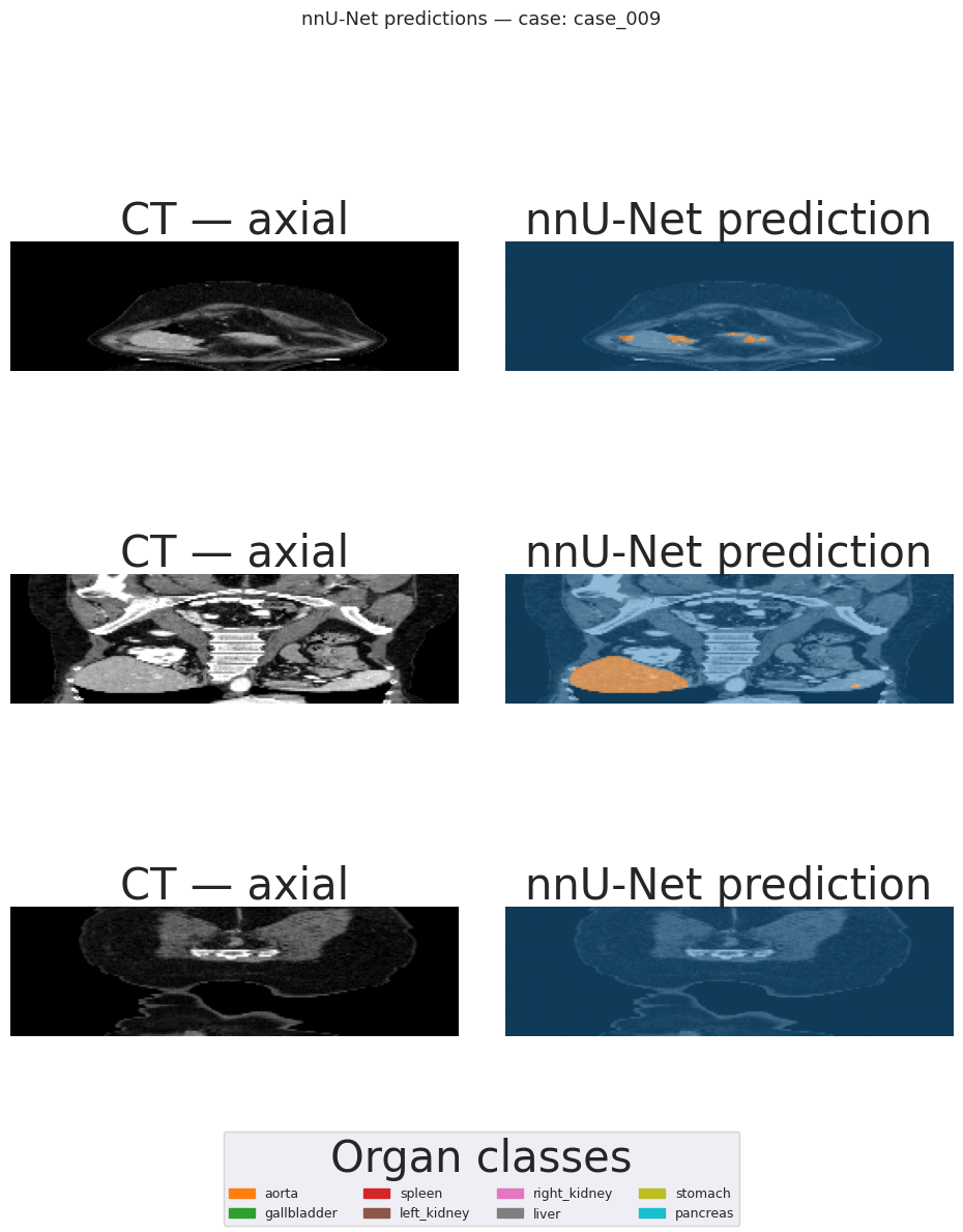
After training, nnU-Net writes test-set predictions to {output_folder_base}/predictions_test/ as NIfTI label maps. Each integer value in the label map corresponds to an organ class (matching the SYNAPSE_CLASSES dict defined below).

The cell below loads up to two test cases, displays three axial slices per case, and overlays the predicted segmentation on the raw CT.

%matplotlib inline
from pathlib import Path

import matplotlib.pyplot as plt
import nibabel as nib
import numpy as np

bridge = results['bridge']
pred_dir = Path(bridge.output_folder_base) / 'predictions_test'
pred_files = sorted(pred_dir.glob('*.nii.gz')) if pred_dir.exists() else []

if not pred_files:
    print(
        "No predictions found.\n"
        "Make sure a 'test' split was assigned before training and that training completed.\n"
        f"Expected prediction dir: {pred_dir}"
    )
else:
    # Locate the exported test images so we can display CT + prediction side-by-side.
    # The exporter writes them to: nnunet_work_dir/raw/Dataset{id}_{name}/imagesTs/
    raw_dir = trainer.nnunet_work_dir / 'raw'
    dataset_dir = min(raw_dir.glob('Dataset*'))
    imagesTs_dir = dataset_dir / 'imagesTs'

    SYNAPSE_CLASSES = {
        1: 'aorta', 2: 'gallbladder', 3: 'spleen',
        4: 'left_kidney', 5: 'right_kidney', 6: 'liver',
        7: 'stomach', 8: 'pancreas',
    }
    num_classes = len(SYNAPSE_CLASSES)
    CMAP = plt.get_cmap('tab10', num_classes + 1)

    for pred_path in pred_files[:1]:  # show at most 2 cases to keep the notebook manageable
        case_id = pred_path.name.replace('.nii.gz', '')
        # Test images are stored as {case_id}_0000.nii.gz (channel-0 suffix added by exporter)
        img_path = imagesTs_dir / f'{case_id}_0000.nii.gz'

        pred_nii = nib.load(str(pred_path))
        pred_vol = pred_nii.get_fdata().astype(np.int32)

        if img_path.exists():
            ct_vol = nib.load(str(img_path)).get_fdata()
        else:
            ct_vol = np.zeros_like(pred_vol, dtype=np.float32)

        # nnU-Net uses (H, W, D) orientation; pick 3 evenly-spaced axial slices
        D = pred_vol.shape[2]
        slice_indices = [D // 4, D // 2, 3 * D // 4]

        fig, axes = plt.subplots(len(slice_indices), 2, figsize=(10, 4 * len(slice_indices)))
        fig.suptitle(f'nnU-Net predictions — case: {case_id}', fontsize=13)

        for row, s in enumerate(slice_indices):
            ct_slice   = ct_vol[:, :, s]
            pred_slice = pred_vol[:, :, s]

            axes[row, 0].imshow(ct_slice, cmap='gray')
            axes[row, 0].set_title('CT — axial')
            axes[row, 0].axis('off')

            axes[row, 1].imshow(ct_slice, cmap='gray')
            axes[row, 1].imshow(pred_slice, cmap=CMAP, alpha=0.5, vmin=0, vmax=num_classes)
            axes[row, 1].set_title('nnU-Net prediction')
            axes[row, 1].axis('off')

        handles = [plt.Rectangle((0, 0), 1, 1, color=CMAP(i + 1)) for i in range(num_classes)]
        labels  = list(SYNAPSE_CLASSES.values())
        fig.legend(handles, labels, loc='lower center', ncol=4, fontsize=9, title='Organ classes')
        plt.tight_layout()
        plt.show()

4. Deployment

The trainer automatically registered a deployment-ready model in MLflow after training. You can deploy it directly to the Datamint server:

job = api.deploy.start(
    model_name=PROJECT_NAME,
    model_alias="latest",
    with_gpu=True,
)

print("Deployment job started!")
print(f"Job ID: {job.id}")
print(f"Status: {job.status}")

Deployment job started!
Job ID: 7daff4f4-caf9-40bd-9584-e417b6600c0f
Status: running

job = api.deploy.get_by_id(job.id)

print(f"Job Status: {job.status}")
print(f"Progress:   {job.progress_percentage}%")

if job.error_message:
    print(f"Error: {job.error_message}")

Job Status: completed
Progress:   100%

Model.is_deployed() reports the same thing, without tracking job IDs, once the job above reaches completed.

registered_model.is_deployed()

4.1 Remote Inference

r = api.resources.get_list(project_name=PROJECT_NAME, limit=1)[0]

inf_job = api.inference.submit(
    model_name=PROJECT_NAME,
    model_alias="latest",
    resource_id=r.id,
)
inf_job.wait()

4.2 Visualise Inference Result

After the inference job completes, the predicted segmentation is uploaded back to the resource as an annotation. The cell below fetches the CT and the predicted segmentation and displays them side by side on three axial slices.

%matplotlib inline
import matplotlib.pyplot as plt
import numpy as np

# Fetch CT volume
ct_nifti = r.fetch_file_data(use_cache=True, auto_convert=True)
ct_vol = ct_nifti.get_fdata()

# Fetch the predicted segmentation (most recent annotation on this resource)
annotations = list(r.fetch_annotations())
pred_ann = annotations[-1]
pred_vol = pred_ann.fetch_file_data(auto_convert=True, use_cache=True)

SYNAPSE_CLASSES = {
    1: 'aorta', 2: 'gallbladder', 3: 'spleen',
    4: 'left_kidney', 5: 'right_kidney', 6: 'liver',
    7: 'stomach', 8: 'pancreas',
}
num_classes = len(SYNAPSE_CLASSES)
CMAP = plt.get_cmap('tab10', num_classes + 1)

# nnU-Net volumes are (H, W, D) — pick 3 axial slices
D = ct_vol.shape[2]
slice_indices = [D // 4, D // 2, 3 * D // 4]

fig, axes = plt.subplots(len(slice_indices), 2, figsize=(10, 4 * len(slice_indices)))
fig.suptitle(f'nnU-Net inference result — {r.filename}', fontsize=13)

for row, s in enumerate(slice_indices):
    ct_slice   = ct_vol[:, :, s]
    pred_slice = pred_vol[:, :, s]

    axes[row, 0].imshow(ct_slice, cmap='gray')
    axes[row, 0].set_title(f'CT — axial slice {s}')
    axes[row, 0].axis('off')

    axes[row, 1].imshow(ct_slice, cmap='gray')
    axes[row, 1].imshow(pred_slice, cmap=CMAP, alpha=0.5, vmin=0, vmax=num_classes)
    axes[row, 1].set_title('nnU-Net Prediction')
    axes[row, 1].axis('off')

handles = [plt.Rectangle((0, 0), 1, 1, color=CMAP(i + 1)) for i in range(num_classes)]
fig.legend(handles, list(SYNAPSE_CLASSES.values()), loc='lower center', ncol=4, fontsize=9, title='Organ classes')
plt.tight_layout()
plt.show()