3D Segmentation with UNETR++ and the Datamint Trainer API

This notebook shows how to train a UNETR++ volumetric segmentation model on the Synapse Multi-Organ CT (https://www.kaggle.com/datasets/dogcdt/synapse) dataset using Datamint’s Trainer API.

What is UNETR++?

UNETR++ (Shaker et al., 2024) is a true 3D segmentation model, it takes full volumetric inputs (B, C, D, H, W) and outputs 3D segmentation maps, unlike slice-based approaches that process 2D cuts independently.

The architecture:

• Encoder: 4-stage hierarchical transformer with Efficient Paired Attention (EPA), decomposes attention into a channel branch and a spatial branch to keep complexity sub-quadratic

• Decoder: 4 transposed-conv blocks with element-wise skip connections; the final block uses a ResBlock (not a transformer) since full-resolution attention is too expensive

Shaker et al., “UNETR++: Delving into Efficient and Accurate 3D Medical Image Segmentation”, IEEE TMI 2024

What You’ll Learn

1. Download and preprocess the Synapse Multi-Organ CT dataset

2. Upload 3D volumes and segmentation masks to Datamint

3. Train with UNETRPPTrainer using a demo-friendly config

4. Visualise 3D predictions on axial slices

Required Dependencies

pip install datamint gdown nibabel h5py

⚠️ Dataset Access

The Synapse dataset can be found at Kaggle.

%pip install -q datamint h5py nibabel

Note: you may need to restart the kernel to use updated packages.

from datamint import Api

PROJECT_NAME = "UNETRPP_Synapse_Tutorial"
api = Api()

1. Setup: Create Project and Load Dataset

Label map (8 abdominal organs):

Value	Organ	Value	Organ
1	aorta	5	right_kidney
2	gallbladder	6	liver
3	spleen	7	stomach
4	left_kidney	8	pancreas

datamint.examples.synapse_dataset downloads the Synapse Multi-Organ CT dataset, converts each HDF5 volume to NIfTI (.nii.gz, downsampled 2x in-plane), and uploads the CT volumes and organ segmentation masks to a Datamint project. The call is idempotent, if the project already exists, it’s returned as-is without re-uploading.

from datamint.examples import synapse_dataset

proj = synapse_dataset.create(project_name=PROJECT_NAME, api=api)
proj

1.1 Assign Train / Val / Test Splits

import random

all_resources = list(api.resources.get_list(project_name=PROJECT_NAME))
all_resources.sort(key=lambda r: r.filename)

random.seed(42)
random.shuffle(all_resources)

n = len(all_resources)
n_train = int(0.70 * n)
n_val   = int(0.15 * n)

api.projects.assign_splits(all_resources[:n_train], split_name='train', project=proj)
api.projects.assign_splits(all_resources[n_train:n_train + n_val], split_name='val', project=proj)
api.projects.assign_splits(all_resources[n_train + n_val:], split_name='test', project=proj)

print(f"Train: {n_train}  Val: {n_val}  Test: {n - n_train - n_val}")

Train: 8  Val: 1  Test: 3

2. Train UNETR++

We use a demo config sized for ≥ 4 GB VRAM.

from datamint.lightning import UNETRPPTrainer

trainer = UNETRPPTrainer(
    project=PROJECT_NAME,
    patch_crop_size=(64, 64, 64),
    feature_size=16,
    num_heads=4,
    depths=[1, 1, 1, 1],
    in_channels=1,
    batch_size=1,
    max_epochs=3,
    sw_overlap=0.5,
    early_stopping_patience=1,
    accelerator='gpu',
)

results = trainer.fit()

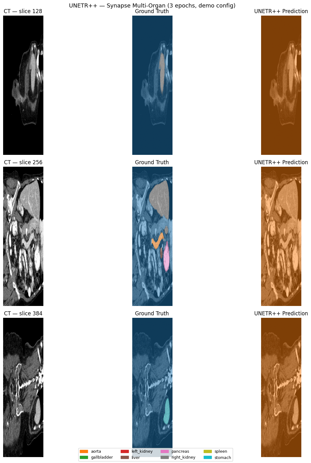
Note on convergence: 3 epochs are enough to verify the pipeline works, but meaningful segmentation quality requires +800 epochs.

print("Test results:")
for metric_dict in results['test_results']:
    for k, v in metric_dict.items():
        print(f"  {k}: {v:.4f}")

Test results:
  test/loss: 1.5252
  test/dice: 0.0025
  test/iou: 0.0002

Inspect the Registered Model

Training automatically registered the model in Datamint’s model registry (backed by MLflow). Use api.models to inspect it without touching MLflow’s client directly:

registered_model = api.models.get_by_name(PROJECT_NAME)
latest_version = registered_model.get_latest_version()

print(f"Version: {latest_version.version}")
print(f"Task type: {latest_version.get_task_type()}")
print(f"Supported modes: {latest_version.get_supported_modes()}")
print("Metrics:")
for metric_name, value in latest_version.get_metrics().items():
    print(f"  {metric_name}: {value}")

3. Visualise Predictions

We pick a test volume, run sliding-window inference, and display a few axial slices with the ground truth and predicted segmentation side by side.

Each colour corresponds to one organ class. The model’s validation_step already uses sliding-window inference internally, here we call it directly for illustration.

import matplotlib.pyplot as plt
import numpy as np
import torch

model = trainer.model
model.eval()

class_names = list(trainer.dataset.seglabel_list)
num_classes  = len(class_names)
print(f'Classes ({num_classes}): {class_names}')

test_ds = trainer.datamodule.test_dataloader().dataset
sample   = test_ds[0]

# Dataset returns numpy arrays: convert before calling model
image    = torch.from_numpy(np.ascontiguousarray(sample['image'])).float()     # (C, D, H, W)
gt_masks = torch.from_numpy(np.ascontiguousarray(sample['masks'])).float()  # (num_classes+1, D, H, W)

with torch.inference_mode():
    logits = model._sliding_window_inference(
        image.unsqueeze(0)  # (1, C, D, H, W)
    )

pred_masks = (logits[0] > 0).cpu()  # (num_classes, D, H, W)

# Collapse to label map: 0 = background, class index + 1 otherwise
gt_np   = gt_masks[1:].numpy()
pred_np = pred_masks.numpy()
gt_label_map   = (gt_np.argmax(axis=0) + 1) * gt_np.any(axis=0)
pred_label_map = (pred_np.argmax(axis=0) + 1) * pred_np.any(axis=0)

# ---- Plot 3 axial slices ----
CMAP = plt.get_cmap('tab10', num_classes + 1)
D = image.shape[1]
slice_indices = [D // 4, D // 2, 3 * D // 4]

fig, axes = plt.subplots(len(slice_indices), 3, figsize=(15, 5 * len(slice_indices)))

for row, s in enumerate(slice_indices):
    ct = image[0, s].numpy()

    axes[row, 0].imshow(ct, cmap='gray')
    axes[row, 0].set_title(f'CT — slice {s}')
    axes[row, 0].axis('off')

    axes[row, 1].imshow(ct, cmap='gray')
    axes[row, 1].imshow(gt_label_map[s], cmap=CMAP, alpha=0.5, vmin=0, vmax=num_classes)
    axes[row, 1].set_title('Ground Truth')
    axes[row, 1].axis('off')

    axes[row, 2].imshow(ct, cmap='gray')
    axes[row, 2].imshow(pred_label_map[s], cmap=CMAP, alpha=0.5, vmin=0, vmax=num_classes)
    axes[row, 2].set_title('UNETR++ Prediction')
    axes[row, 2].axis('off')

handles = [plt.Rectangle((0,0),1,1, color=CMAP(i+1)) for i in range(num_classes)]
fig.legend(handles, class_names, loc='lower center', ncol=4, fontsize=9)
plt.suptitle('UNETR++ — Synapse Multi-Organ (3 epochs, demo config)', fontsize=13)
plt.tight_layout()
plt.show()

Classes (8): ['aorta', 'gallbladder', 'left_kidney', 'liver', 'pancreas', 'right_kidney', 'spleen', 'stomach']

4. Customisation Options

6.1 Production config (paper settings)

trainer = UNETRPPTrainer(
      project=PROJECT_NAME,
      patch_crop_size=(64, 128, 128),
      feature_size=16,
      num_heads=4,
      depths=[3, 3, 3, 3],
      in_channels=1,
      batch_size=2,
      max_epochs=1000,
      sw_overlap=0.5,
      num_workers=4,
      early_stopping_patience=50,
      accelerator='auto',
  )

6.2 Mixed precision (halves VRAM)

trainer = UNETRPPTrainer(
    project=PROJECT_NAME,
    patch_crop_size=(128, 128, 128),
    trainer_kwargs={'precision': '16-mixed'},
)

6.3 Custom loss

from monai.losses import DiceCELoss

trainer = UNETRPPTrainer(
    project=PROJECT_NAME,
    loss_fn=DiceCELoss(to_onehot_y=False, sigmoid=True),
)

6.4 Multi-channel MRI (e.g. BraTS)

trainer = UNETRPPTrainer(
    project='BraTS_Project',
    in_channels=4,   # T1, T1ce, T2, FLAIR
    patch_crop_size=(128, 128, 128),
)

6.5 Sliding-window overlap at inference

Higher overlap reduces stitching artefacts at the cost of more compute. The default is 0.5.

trainer = UNETRPPTrainer(
    project=PROJECT_NAME,
    sw_overlap=0.75,   # more overlap → smoother predictions, ~4× slower
)

5. Deployment

The trainer automatically registered a deployment-ready model in MLflow after training. You can deploy it directly to the Datamint server:

job = api.deploy.start(
    model_name=PROJECT_NAME,
    model_alias="latest",
    with_gpu=False,
)

print("Deployment job started!")
print(f"Job ID: {job.id}")
print(f"Status: {job.status}")

job = api.deploy.get_by_id(job.id)

print(f"Job Status: {job.status}")
print(f"Progress:   {job.progress_percentage}%")

if job.error_message:
    print(f"Error: {job.error_message}")

Model.is_deployed() reports the same thing, without tracking job IDs, once the job above reaches completed.

registered_model.is_deployed()

5.1 Remote Inference

r = api.resources.get_list(project_name=PROJECT_NAME, limit=1)[0]

inf_job = api.inference.submit(
    model_name=PROJECT_NAME,
    model_alias="latest",
    resource_id=r.id,
)
inf_job.wait()